Introduction

Одной из основных целей любого государства является обеспечение доступной, надежной и устойчивой электрической энергией. Главное препятствие к этому связано с тем фактом, что энергоснабжающие организации не всегда обладают всеобъемлющей картой воздушных линий электропередач, а схемы, которые существуют, как правило, устарели и неполны. Без централизованной карты, правительства или другие организации не обладают знаниями для принятия обоснованных решений об инвестировании средств в техническое обслуживание или расширение электрической сети. Этот недостаток информации также усложняет принятие решений об установке альтернативных источников энергии – не зная, где обычная сеть, трудно разумно использовать альтернативы, такие как солнечная или ветровая энергия. Помимо самой карты, правительства и организации нуждаются в быстром и экономически эффективном инструменте. Высоковольтная сеть постоянно расширяется, поэтому важным моментом является возможность создания точных снимков через равные промежутки времени. Функционал платформы cGIS включает алгоритм, способный эффективно картировать инфраструктуру воздушных линий электропередач.

This feature provides an automatic solution to the problem of power line detection based on the use of machine learning. The solution is an algorithm that receives remote sensing data as input. The resulting images are processed in the visible spectrum by a neural network and return geospatial locations that with a high degree of probability contain elements of high-voltage infrastructure - power line poles. This data further requires verification by the operator. However, even in their original form, they are classified as geographic positions that correspond with a high degree of probability to the locations of real objects in the areas.

Classification or detection?

The first question to create such a solution was to set the machine learning task itself. We were initially inspired by the way DevSeed solved a similar problem. Their solution involves the classification of vector tiles, on a map with a scale of 1:2000, which indicates whether there are power line poles on a given tile. Subsequently, the operator needs to manually trace power lines on the classified tiles, using a web interface with an interactive map.

This method of overhead power lines recognition has proved to be insufficiently effective. We decided to find a better solution to this problem, namely the direct detection of the power poles themselves on the map.
 
We decided to use detection instead of classification because the detection algorithm has the same disadvantages as the classification algorithm.

Advantages:

1. Strong approximation (1:2000) is not required to detect power lines. Publicly available maps at scales larger than 1:4000 require a special rate plan, while for detection the size of the tile is not essential, it is only important that the power line pole itself is directly distinguishable on the map.
2. The manual tracing process is not required.
3. The detection output immediately gives the location of the power line pole in geographic coordinates, allowing the power lines to be traced automatically.

Disadvantages:

1. False positives when trees can stand out as power line poles.
2. Misses, when some objects on the map may be missed due to an error in the detection algorithm.

Raw data for machine learning

The input data for the training task are the geographic coordinates of power line poles categorized by the following meaningful attributes: pole type, product material, voltages, and others. A total of 211725 objects were represented in the full dataset. Further work was carried out with the data grouped by support type as the most representative feature. The following is a summary of the data by this criterion.

Due to the lack of distinguishability of objects of all designated types on the images, the following objects were selected for further work in the machine learning algorithm:

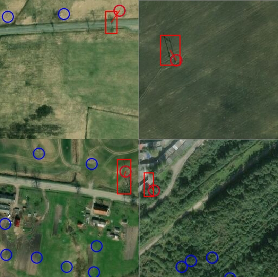
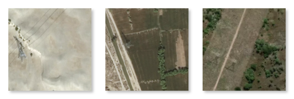
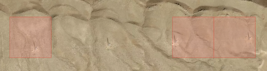
The data for machine learning was a raster image of 512x512 pixels with the areas of high-voltage power line towers marked on it. The markup was a rectangular area in the image, corresponding to an average area of 70x70 meters on the ground.

For machine learning, the original raster images were partitioned with 80% data for training and 20% data for testing.

Choice of solution architecture

For the task of detecting objects in an image where objects of the target class are only a small part of the image, it is a problem that the parts of the image where the target object is missing contribute too much to the training process, eventually leading to many gaps in the test set. To solve this problem, we used the Focal Loss neural network function, which reduces the influence of frequent backgrounds and increases the importance of infrequent objects in training.

Thus, the following neural network architecture for detection was chosen - RetinaNet, which just uses Focal Loss as the loss function.

During the RetinaNet training, the loss function is calculated for all considered orientations of candidate areas (anchors), from all levels of image scaling. In total, there are about 100 thousand areas for one image. The Focal Loss value is calculated as the sum of function values for all anchors, normalized by the number of anchors containing the sought objects. The normalization is done only by them and not by the total number, since the vast majority of anchors are easily defined backgrounds, with little contribution to the total loss function.

Structurally, RetinaNet consists of Backbone and two additional networks (Classification Subnet) and Object Boundary Definition (Box Regression Subnet).

The so-called Feature Pyramid Network (FPN), which operates on top of one of the commonly used convolutional neural networks (e.g. ResNet-50), is used as the basis neural network. FPN has additional lateral outputs from hidden layers of the convolutional network, forming pyramid levels with different scales. Each level is supplemented with "knowledge from above", i.e. information from the higher levels, which are smaller in size but contain information about areas of the larger area. It looks like artificial enlargement (for example, by simple repetition of elements) of more "collapsed" feature map to the size of the current map, their element-by-element summation, and transfer both to lower levels of the pyramid and input of other subnets (i.e. to Classification Subnet and Box Regression Subnet). This allows extracting from the original image a pyramid of features at different scales, on which both large and small objects can be detected. FPN is used in many architectures, improving the detection of objects of different scales - RPN, DeepMask, Fast R-CNN, Mask R-CNN, and others.

Our network, like the original one, uses FPN with 5 levels numbered P3 through P7. The level Pl has a resolution 2l times smaller than the input image. All levels of the pyramid have the same number of channels C = 256 and the number of anchors.

The areas of the anchors were chosen as follows: [16 x 16] to [256 x 256] for each pyramid level from P3 to P7, respectively, with an offset step (strides) of [8 - 128] pixels. This size allows analyzing small objects and some surrounding areas. In our case, these are power line poles with their surrounding shadows.

Training and Results

Machine learning results were evaluated in the following ways:

1. Testing on a delayed sample of 20% of the original sample to match the predicted rectangular frames and the true manually marked ones by the expert. 70% of the rectangle areas were correctly identified, given that the amount of data is not numerous.
2. Calculating the deviation distance of the actual coordinates from the predicted coordinates in the entire dataset. During the automatic location of the supports by the machine-learning algorithm, up to 60% of the locations were found to correspond to the actual objects of the electrical networks (supports) and are, on average, at a distance of no more than 70 meters from the predicted ones. Also, there were found cases when there were no poles in the data, but the algorithm found them in the image, which eventually led to a distortion of the quality metric, because there is an object in the image, but it is not in the reference database, which suggests that the algorithm can be successfully used to update the databases with information about power lines.