We faced the task of analyzing the movement of pedestrians and vehicles to automatically obtain various data based on the analysis of image sequences from surveillance cameras in real-time or archived records. For this purpose, we used special software allowing us to control and analyze the data in automatic mode. For our case, we developed a system for monitoring vehicle and pedestrian traffic on the roads to assess traffic congestion and subsequent optimization of traffic flow through the GIZMOre/cGIS platform functionality.
We took data from surveillance cameras that provide video streams from several intersections in the city.
Each camera provides:
To analyze traffic it is necessary to obtain data on the movement of people and vehicles in the area covered by the cameras and to build statistics based on counting the number of occurrences of a particular class of object.
But it is not enough just to count the appearances of objects to make an objective assessment of traffic congestion. It is necessary to understand the spatial distribution of congestion, i.e. what road segments are congested in terms of geospatial coordinates.
With the presence of the trajectories of traffic and people, it becomes possible to build heatmaps of traffic congestion to visualize it on the electronic map.
Thus, for the task we need to solve the following subtasks:
Parallel processing of data from multiple cameras was decided to be performed using Apache Kafka, which allows the creation of a queue of frames for each surveillance camera. Frames from each camera are processed by the ffmpeg library, namely:
It is worth to note, that the use of ffmpeg for storyboarding is justified by the fact that OpenCV has no functionality for the processing of byte messages from the RAM.
Для решения задачи детектирования было решено использовать модель семейства YOLO. Модели данного семейства хорошо показали себя для решения задач обнаружения объектов в реальном времени в соревнованиях VOC, ImageNet Classification Challenge и многих других.
At the time of writing this article, the most optimal model is YOLOv3 and its variations. Two architectures will be discussed next: YOLOv3 and Tiny YOLOv3. The second architecture is a simplified implementation of the YOLOv3 model to speed up performance and get more frames per second (FPS).
To solve the problem of object tracking and identification, we chose between SORT and DeepSORT algorithms.
The essence of the SORT algorithm is to use a Kalman filter to operate the tracker. The basic idea of the Kalman filter is that the detector, no matter how good it is in quality on the validation sample, may at some point not detect an object due to occlusions, poor visibility, or remoteness. Nevertheless, the motion of each object can be estimated using a kinematic model based on previous estimates. Thus, we first obtain the most probable estimate of the object's position and then refine it when the estimates from our detector appear.
The problem, in this case, remains object identification, that is, determining that it was the same object in the previous frame.
This is usually achieved by measuring the distance between the centroids of the rectangular frames obtained by the detector (Figure 1). We assume that the same object will be at a minimum distance between the closest frames, but this does not work in all cases.
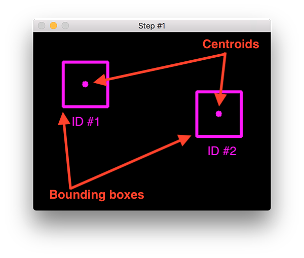
For example, two people walking towards each other, and after their intersection in the frame may mix up the identifiers of these objects, which will lead to errors.
For this purpose, the SORT algorithm is modified by adding a separate neural network that converts part of the image in the frame predicted by the detector into a fixed-length vector that describes the semantic meaning of the image with the property of distance, that is, the distance between two such vectors tells the degree of similarity of objects in the image.
This is achieved by training the neural network to the distance metric, showing similar and dissimilar pairs in the training. The output is a neural network that converts the image into a vector with the distance property.
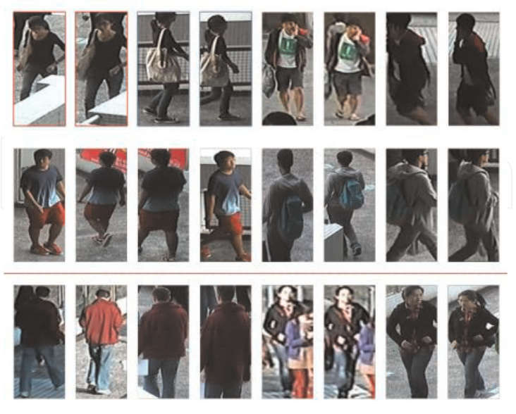
We obtain DeepSORT algorithm, which compares not the distance between centroids of rectangular frames on different frames, but their semantic descriptions. In this way, object identification becomes more robust to errors of the false-positive type.
The problem with this approach is the fact that the neural network constructing semantic vectors must do so for a certain class of objects, for example, for people, cars, trucks. Therefore, to track both cars and people in the same frame, we need two trained encoders (a neural network that converts the image into a semantic vector) for people and vehicles.
In solving our problem, we used ready-made weights for the YOLOv3 detector, which recognizes 80 classes from the VOC dataset. For the default encoder, we used weighting coefficients pre-trained to encode semantic vectors for people on the Market-1501 dataset.
Since we also need to track cars, we added the task of training the encoder for objects of the class of cars.
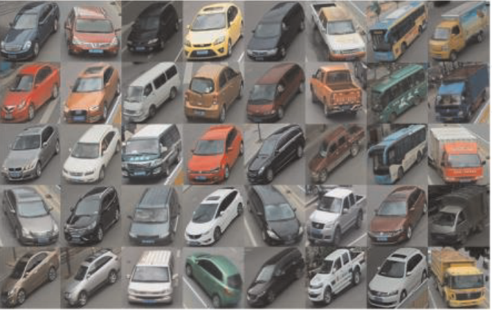
To train the encoder to transform images with vehicles, we used the VeRi dataset containing images pairs (X - Y), where
A total of 40 thousand images, where for each image there is at least one pair.
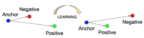
Based on the available pairs, triplets are constructed, that is, for the pair (X - Y) (anchor - positive), image Z (negative) is selected, which contains an object, not similar to those contained in the pair (X - Y). Thus, a triplet loss function is formed to train vectors of similar objects to be close and different objects to be far away from each other.
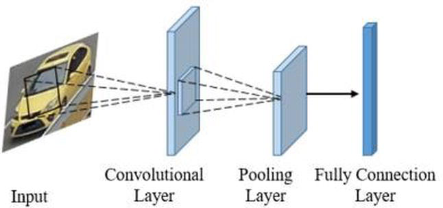
To encode images into a semantic vector we used a small convolutional neural network, consisting of 3 convolutional layers, and pooling layers between them. At the end, there was a fully connected layer of size 128.
The training was performed using TensorFlow machine learning framework on an Nvidia GeForce 1660 TI 6 GB video card:
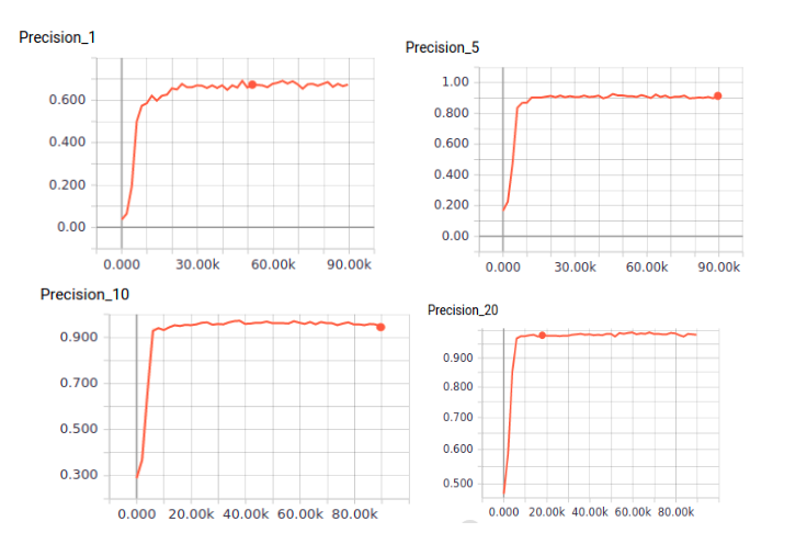
The quality was evaluated using Precision@k quality metric. This metric is used to assess the quality of search engines. If you query for a particular image, the Precision@k metric gives the probability of the required object appearing in the sample of k images in the query.
So we got the following results:
| Metric | Value |
| Precision@1 | 0.69 |
| Precision@5 | 0.91 |
| Precision@10 | 0.94 |
| Precision@20 | 0.98 |
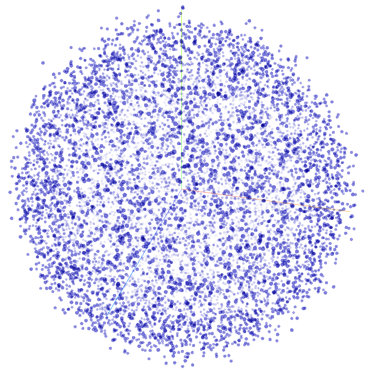
If we use vector dimensionality reduction algorithms (such as t-SNE) computed for all 40 thousand images, we can display all cars in a semantic 3D space, where the most similar objects are located closest to each other (Figure 7).
The result was a lightweight neural network capable of transforming the image into a vector, which has the property of distance. The smaller the distance between the vectors, the more similar the objects in the image are to each other.
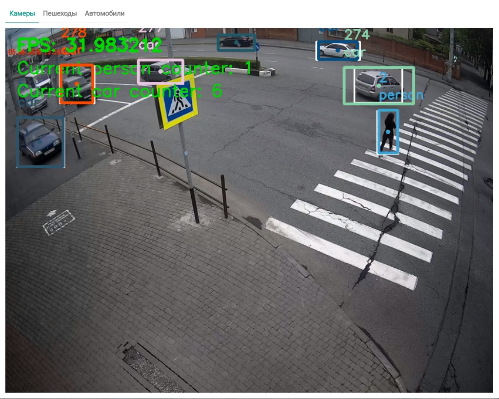
By incorporating this neural network into the tracker algorithm, we were able to detect the traffic of many objects of different classes, namely people and vehicles (Figure 8).
Once we have the algorithm for tracking objects in the video stream, we faced the task of learning how to display the trajectories of objects on the map to further calculate the traffic volume and degree of congestion in a given time interval.
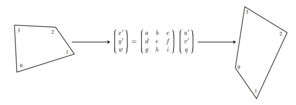
To begin with, we applied a perspective transformation. That is, on each camera of interest we marked edge pixels at each corner of the image on the condition that we can find objects attached to these pixels on the map. This allows us to transfer the objects in the camera plane to the Earth's surface plane by matching the points on the camera plane with the corresponding points on the Earth's surface (Figure 9).

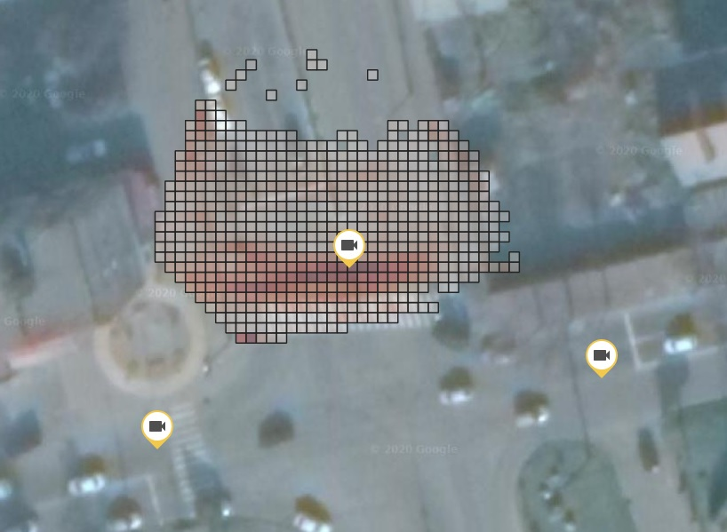
By marking the pixels, we found the landmarks attached to them on the map and determined their geographic coordinates in latitude/longitude format.
Then, the pixels on the camera were converted into points on the map through perspective transformation, and the obtained trajectories of the objects were transferred to the Earth plane (Figure 10).
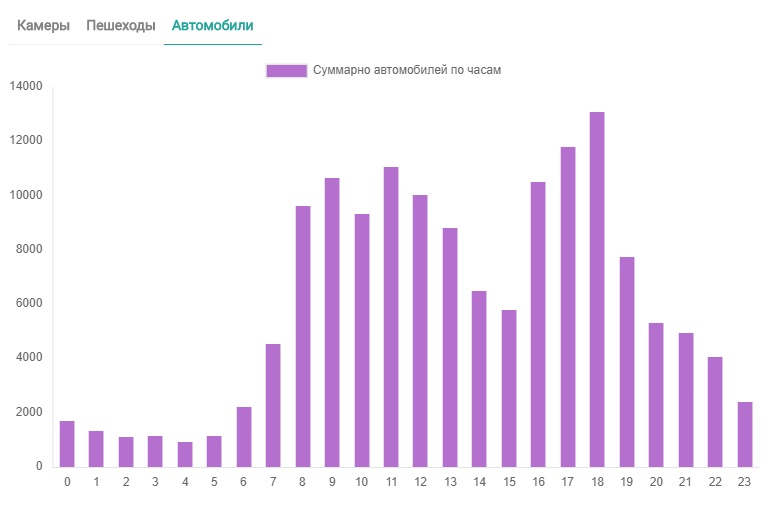
Based on the obtained trajectories and the frequency of the appearance of objects, we built heatmaps of the movement of objects and built histograms of the appearance of objects in one or another part of the city, where the cameras were installed.

The next task was to optimize the tracking algorithms for real-time use. Since we need to process multiple cameras with the least amount of resources, we need to use all possible tools to speed up the neural networks.
In the first iteration, when the model was run, the number of frames per second for one camera did not exceed 11 FPS, that is, the model in its original form was too heavyweight and could not be used for real-time work.
At first, we tried to process only every 4th frame of the video stream, which gave a linear increase in performance. That is, by reducing the number of frames by n times we got an n-fold performance gain in the model. The algorithm started to work with a 40-45 FPS frame rate. But this still wasn't enough, because adding more and more cameras reduced speed in the same way, which reduced this improvement to processing only two cameras on one server.
Then we decided to change the architecture of the detector, but retain its basic idea by applying the Tiny YOLOv3 model.
Tiny YOLOv3 significantly improved the speed of video stream processing, so we could process 8 cameras at 30 FPS.
Subsequent improvements were already related to cost optimization. It is known that using rented servers with video cards is an extremely expensive service, so we decided to look at existing optimization tools for detecting algorithms on Intel processors.
We considered Intel's OpenVino Toolkit framework as an optimization tool. Using this tool, we optimized our model for Intel processors and experimented with different configurations.
| Experiment number | Number of video streams | Number of virtual threads (vCPU) | FPS |
| 1 | 4 | 2 | 20 |
| 2 | 4 | 4 | 35 |
| 3 | 4 | 8 | 40 |
| 4 | 8 | 2 | 18 |
| 5 | 8 | 4 | 22 |
| 6 | 8 | 8 | 25 |
| 7 | 16 | 2 | 10 |
| 8 | 16 | 4 | 12 |
| 9 | 16 | 8 | 15 |
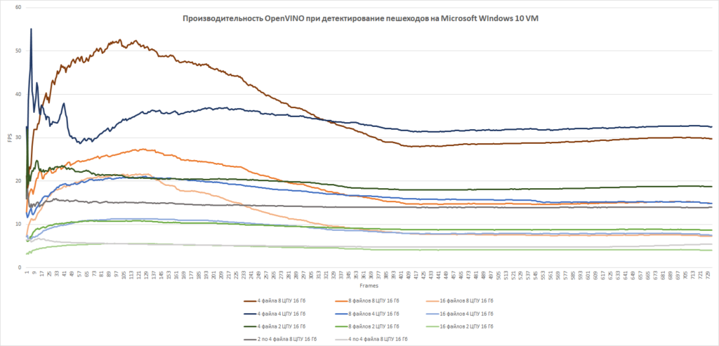
Based on our experiments we have selected a stable configuration for processing video streams from 8 cameras on 8 vCPU, which further allowed us to scale the solution with optimal server architecture in terms of budget.
This article describes the research and development cycle of the solution for analyzing video streams from surveillance cameras and obtaining traffic and pedestrian analysis. The developed technology stack allowed us to further create other solutions in this area using modern technologies in the field of artificial intelligence.